



You’ve captured 400 drone images of a construction site with your RTK-equipped Mavic 3 Enterprise. The photogrammetric point cloud is done — solid, validated, survey-grade. But the client also wants an immersive 3D walkthrough for the project stakeholders who don’t read point clouds. You’ve heard NeRF can do that. The question is whether you can build one that actually ties to real-world coordinates — not just a pretty floating scene in arbitrary space.
The answer is yes. But not out of the box, and not without understanding where the georeferencing actually lives in the pipeline. Every NeRF framework — Nerfstudio, Instant NGP, Luma AI — operates in scene-local coordinates by default. Getting from scene-local to WGS84 or a projected CRS requires deliberate steps at capture, processing, and export. Skip any of them and you get a visually impressive model that can’t be placed on a map.
This tutorial walks through the full workflow: capture requirements, COLMAP geo-registration, Nerfstudio training, georeferenced export, and accuracy validation. The pipeline has been validated on sites ranging from roughly 0.5 to 4 hectares. It works — with caveats worth being specific about.
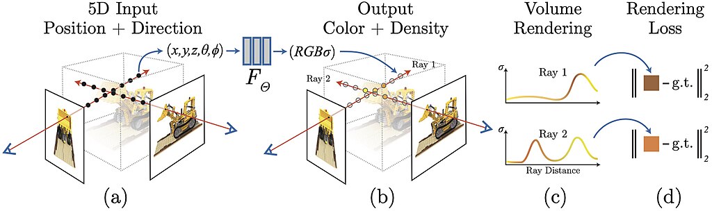 Mildenhall et al. (2020), from the original NeRF paper repository, MIT License
Step 1: Plan the Drone Capture for NeRF
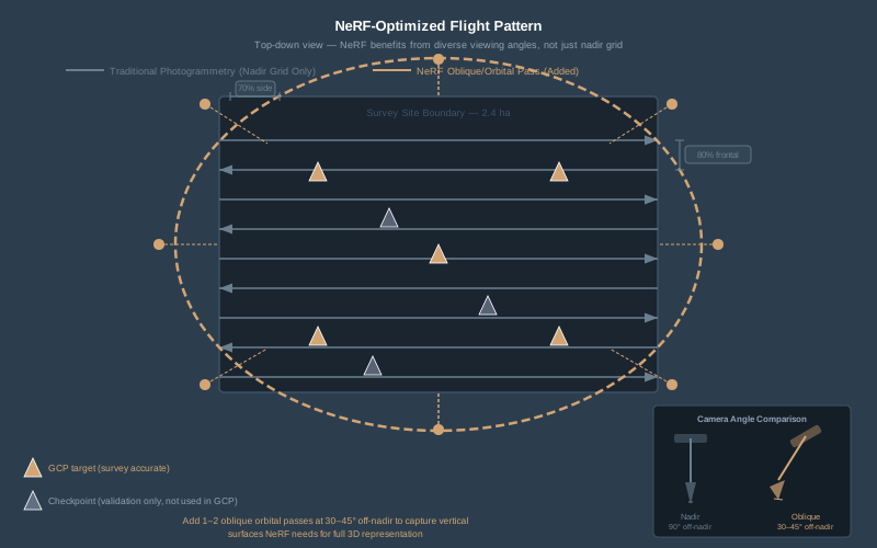
NeRF reconstruction is not the same as photogrammetric reconstruction, and your flight plan needs to reflect that. Traditional photogrammetry wants consistent nadir imagery with controlled overlap. NeRF wants diverse viewing angles — the more varied the perspectives, the better the volumetric representation.
Flight parameters that matter:
- Overlap. 80% frontal, 70% side — minimum. NeRF is more sensitive to coverage gaps than photogrammetry because it needs to reconstruct view-dependent appearance, not just geometry. At 60% frontal overlap, COLMAP will reconstruct camera poses but the NeRF will have artifacts in under-observed regions.
- Oblique passes. Fly at least one orbital or crosshatch pass at 30-45 degrees off nadir. This is where NeRF pulls ahead of traditional photogrammetry for visualization — oblique views capture vertical surfaces (building facades, retaining walls, cut slopes) that nadir-only missions miss entirely. Two oblique passes at different altitudes is better.
- Altitude. 60-90 meters AGL for site-scale scenes (2-5 hectares). Lower is higher resolution but exponentially more images. At 75m AGL with a Mavic 3 Enterprise (12.8mm lens), ground sampling distance is roughly 2 cm/pixel — more than sufficient for NeRF training.
- Exposure. Manual or shutter priority. NeRF is sensitive to exposure variation between frames — auto-exposure creates inconsistent lighting that the network interprets as view-dependent effects rather than what it actually is: your camera hunting. Lock ISO, set shutter speed for the conditions, and let it ride.
- Image count. 300-800 images for a 2-5 hectare site. More images means longer COLMAP processing and longer training but better reconstruction. Under 200 images and COLMAP starts struggling with feature matching on large outdoor scenes.
RTK or PPK geotagging is non-negotiable. If you want georeferenced output, you need georeferenced input. Autonomous phone-GPS geotags at 2-5 meter accuracy are useless for anything beyond rough scene placement. RTK gives you 1-3 cm positions in the EXIF data; PPK gives you the same after post-processing. Either works. The positions don’t need to be perfect — they need to be consistent and in a known datum.
Common combinations: DJI Mavic 3 Enterprise with RTK for urban sites, and PPK post-processing with an Emlid RS3 base for remote work. Both produce usable geotags for this pipeline.
Step 2: Set GCPs for Georeferencing and Validation
Ground control points serve two purposes in a NeRF workflow: they anchor the COLMAP reconstruction to real-world coordinates, and they give you something to validate against after export.
GCP target design. Standard photogrammetry targets work fine — 12x12 inch checkerboard or circular coded targets, high contrast against the ground surface. NeRF doesn’t need anything special because the GCPs are consumed by COLMAP during Structure-from-Motion, not by the neural network itself. The SfM engine sees them the same way it sees any other feature point.
Distribution. Five GCPs minimum for georeferencing — corners and center of the site, well-distributed in X, Y, and Z. If you have significant terrain variation, get a GCP at your highest and lowest elevations. Then place 3-5 additional points as independent checkpoints — these are not used in the georeferencing step. They exist solely to validate accuracy after export.
Survey method. RTK rover on a known control network, or PPK observations with 180-second occupations on each point. Record in the project datum — if the deliverable is NAD83/State Plane, survey your GCPs in NAD83/State Plane. Datum transformations at the GCP stage introduce error that propagates through the entire pipeline.
Record the coordinates in a text file. You’ll need them in COLMAP’s model_aligner format later:
GCP_01.jpg 425789.123 4512301.456 312.78
GCP_02.jpg 425812.456 4512289.012 311.92
GCP_03.jpg 425801.789 4512315.678 313.45
If you’re using geographic coordinates (lat/lon/ellipsoidal height), that works too — COLMAP converts internally.
Step 3: Process Camera Poses with COLMAP
COLMAP is the backbone. Every NeRF framework that works with arbitrary image sets uses COLMAP (or a fork of it) to estimate camera poses through Structure-from-Motion. The quality of your NeRF lives and dies with the quality of your COLMAP reconstruction.
Install COLMAP 4.x. As of early 2026, the pose_prior_mapper (introduced in COLMAP 4.0) directly integrates GPS priors during reconstruction — a significant improvement over the old workflow of reconstructing first and aligning second.
Option A: GPS-Prior Reconstruction (Recommended)
If your images have RTK/PPK coordinates in the EXIF data, COLMAP 4.x can use them as pose priors during the reconstruction itself. This is cleaner than the legacy two-step approach.
# Feature extraction — COLMAP reads GPS from EXIF automatically
colmap feature_extractor \
  --database_path project/database.db \
  --image_path project/images \
  --ImageReader.camera_model OPENCV \
  --ImageReader.single_camera 1

# Feature matching
colmap exhaustive_matcher \
  --database_path project/database.db \
  --SiftMatching.guided_matching 1

# Reconstruction with GPS pose priors
colmap pose_prior_mapper \
  --database_path project/database.db \
  --image_path project/images \
  --output_path project/sparse \
  --PosePrior.prior_position_std_x 0.03 \
  --PosePrior.prior_position_std_y 0.03 \
  --PosePrior.prior_position_std_z 0.05
The prior_position_std values tell COLMAP how much to trust your GPS positions. For RTK-fixed positions, 0.03 meters (3 cm) horizontal and 0.05 meters (5 cm) vertical is realistic. For PPK-processed positions, same values. For phone GPS, use 3.0-5.0 meters — but at that point, you’re not really georeferencing.
Option B: Reconstruct Then Align (Legacy Workflow)
If your COLMAP version doesn’t support pose_prior_mapper, or you want more control over the alignment:
# Standard reconstruction
colmap automatic_reconstructor \
  --workspace_path project \
  --image_path project/images

# Geo-register using GPS coordinates
colmap model_aligner \
  --input_path project/sparse/0 \
  --output_path project/sparse/0_georef \
  --ref_images_path project/gcp_coordinates.txt \
  --ref_is_gps 1 \
  --alignment_type ecef \
  --alignment_max_error 3.0
The model_aligner computes a 3D similarity transformation (rotation, translation, scale) between COLMAP’s arbitrary coordinate system and your real-world coordinates. It uses RANSAC internally, so outliers in your GCP list get rejected — but you still want clean input. Three reference points is the minimum; five or more is standard practice.

Verify the reconstruction. Open the sparse model in COLMAP’s GUI. Check that all cameras registered (compare image count in vs. registered count). If more than 5% of images failed to register, your overlap was insufficient or there’s a lighting/exposure problem in a section of the flight. Look at the sparse point cloud — it should roughly match your site geometry. If it looks like abstract art, something went wrong.
Step 4: Convert to Nerfstudio Format and Train
Nerfstudio is the most accessible open-source framework for training NeRFs from arbitrary image sets. It reads COLMAP output directly.
# Convert COLMAP output to Nerfstudio format
ns-process-data images \
  --data project/images \
  --output-dir project/nerfstudio \
  --colmap-model-path project/sparse/0_georef \
  --skip-colmap
The --skip-colmap flag tells Nerfstudio to use your existing COLMAP reconstruction instead of running its own. This is critical — you already did the georeferenced reconstruction in Step 3. Letting Nerfstudio re-run COLMAP would throw away your geo-registration.
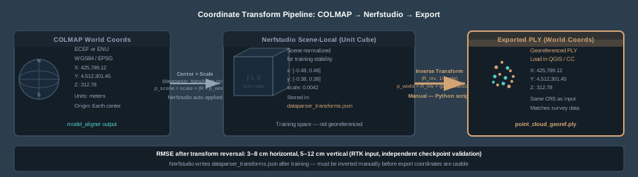
This produces a transforms.json file containing camera poses in Nerfstudio’s coordinate convention (OpenGL: +X right, +Y up, +Z back). The conversion from COLMAP’s OpenCV convention (+X right, +Y down, +Z forward) is handled automatically. But here’s the detail that matters for georeferencing: Nerfstudio also applies a centering transform and scale factor to normalize the scene into a unit cube. These transforms are stored in dataparser_transforms.json after training. You need them later to reverse-transform your exports back to real-world coordinates.
Choose Your Method
# Nerfacto — general purpose, good quality, reasonable speed
ns-train nerfacto --data project/nerfstudio

# Splatfacto — 3D Gaussian Splatting, faster training and real-time rendering
ns-train splatfacto --data project/nerfstudio

# Instant-NGP — fastest training, lower quality on large scenes
ns-train instant-ngp --data project/nerfstudio
For drone survey scenes, I use Nerfacto when I need the highest geometric quality for point cloud export, and Splatfacto when the deliverable is a real-time viewer for stakeholder presentations. Instant-NGP trains in minutes but the geometry on large outdoor scenes doesn’t hold up for measurement.
Training time. Nerfacto on a 500-image drone dataset: 2-4 hours on an RTX 4090, 6-10 hours on an RTX 3080. Splatfacto is faster — roughly half. Plan accordingly.
Step 5: Export Georeferenced Products
This is where most tutorials stop, and where the actual work of georeferencing begins.
Nerfstudio exports point clouds and meshes in scene-local coordinates — the normalized unit-cube space it used during training. To get back to real-world coordinates, you need to reverse the transforms that Nerfstudio applied.
Export the Point Cloud
# Export dense point cloud as PLY
ns-export pointcloud \
  --load-config outputs/project/nerfacto/config.yml \
  --output-dir exports/ \
  --num-points 1000000 \
  --remove-outliers True \
  --normal-method open3d
Export a Mesh
# Export textured mesh using TSDF fusion
ns-export tsdf \
  --load-config outputs/project/nerfacto/config.yml \
  --output-dir exports/ \
  --target-num-faces 500000 \
  --resolution 512
Reverse the Dataparser Transforms
The exported PLY is in Nerfstudio scene-local space. To recover real-world coordinates:
- Read
dataparser_transforms.jsonfrom the training output directory. It contains a 3x4 transform matrix and a scale factor. - Invert the transform. Every point in the exported PLY was transformed as:
p_scene = scale * (R * p_world + t). To reverse:p_world = R_inv * (p_scene / scale - t). - Apply the inverse to every point in the PLY file.
Here’s a Python script that does this:
import numpy as np
import json
from plyfile import PlyData, PlyElement

# Load the dataparser transforms
with open("outputs/project/nerfacto/dataparser_transforms.json") as f:
    meta = json.load(f)

transform = np.array(meta["transform"])  # 3x4 matrix
scale = meta["scale"]

# Extract rotation and translation
R = transform[:3, :3]
t = transform[:3, 3]
R_inv = np.linalg.inv(R)

# Load exported PLY
ply = PlyData.read("exports/point_cloud.ply")
points = np.vstack([
    ply["vertex"]["x"],
    ply["vertex"]["y"],
    ply["vertex"]["z"]
]).T

# Reverse transform: scene-local → world coordinates
points_world = (R_inv @ (points / scale - t).T).T

# Overwrite coordinates
ply["vertex"]["x"] = points_world[:, 0].astype(np.float32)
ply["vertex"]["y"] = points_world[:, 1].astype(np.float32)
ply["vertex"]["z"] = points_world[:, 2].astype(np.float32)

ply.write("exports/point_cloud_georef.ply")
print(f"Exported {len(points_world)} points in world coordinates.")
If your COLMAP reconstruction was geo-registered in ECEF coordinates, the output PLY is now in ECEF. If you aligned to a local ENU frame or a projected CRS, it’s in that frame. Know your coordinate system — it’s whatever you fed into model_aligner.
Step 6: Alternative Paths — Luma AI and Pix4Dcloud
Not every project justifies the open-source pipeline. Two commercial alternatives handle parts of this workflow with less friction.
Luma AI
Luma captures scenes from phone video or uploaded images and produces Gaussian Splats viewable in-browser. The catch: zero georeferencing. Exports come as PLY or GLB files in arbitrary local coordinates with no connection to any CRS. You can load a Luma PLY into QGIS, but it lands at the origin with no spatial reference.
Luma is useful for quick stakeholder visualization — “here’s what the site looks like in 3D” — but not for any workflow that requires the model to sit on a map or align with survey data. Treat it as a visualization tool, not a measurement tool.
Pix4Dcloud with Georeferenced Gaussian Splatting
As of late 2025, Pix4Dcloud introduced georeferenced Gaussian Splatting for drone imagery. This is the closest thing to a turnkey solution: upload your drone images (with RTK geotags), and Pix4D runs its standard photogrammetric pipeline — bundle adjustment, densification, meshing — and now adds a Gaussian Splat output that inherits the same georeferencing as the point cloud and mesh.
The splats are fully georeferenced, viewable alongside traditional photogrammetric products in the Pix4Dcloud viewer, and exportable. For operators already in the Pix4D ecosystem, this is the path of least resistance. The tradeoff is cost ($399/month for Pix4Dmapper, cloud processing credits on top) and the fact that you’re locked into Pix4D’s pipeline with limited control over the splatting parameters.
Step 7: Validate Accuracy Against Survey Checkpoints
You built the NeRF, exported the point cloud, reversed the transforms. Now prove it’s accurate. Without validation, you have a pretty model with unknown positional quality.
Pull checkpoint coordinates. These are the 3-5 survey points you set in Step 2 that were not used in the COLMAP geo-registration. They should be visible in the exported point cloud as distinct targets on the ground surface.
Measure the NeRF-derived positions. Load the georeferenced PLY in CloudCompare, QGIS, or your point cloud viewer of choice. Identify each checkpoint target and record its XYZ coordinate from the NeRF point cloud.
Compute RMSE. For each checkpoint:
error_x = nerf_x - survey_x
error_y = nerf_y - survey_y
error_z = nerf_z - survey_z
horizontal_error = sqrt(error_x^2 + error_y^2)
Then:
RMSE_horizontal = sqrt(mean(horizontal_error^2))
RMSE_vertical = sqrt(mean(error_z^2))
What to expect. Based on current research and my own testing:
| Metric | NeRF (RTK/PPK input) | Traditional Photogrammetry |
|---|---|---|
| Horizontal RMSE | 3-8 cm | 1-3 cm |
| Vertical RMSE | 5-12 cm | 2-5 cm |
| Point cloud noise | Moderate (wavy surfaces on flat areas) | Low |
| Texture quality | Superior for complex geometry | Good for nadir-visible surfaces |
NeRF point clouds carry 2-3x more geometric noise than photogrammetric MVS point clouds on the same datasets. A 2025 comparative study (Tanaka et al., International Journal of Automation Technology) found that NeRF-reconstructed point clouds “contain substantial noise and show wavy surfaces even on flat surfaces.” That matches my field experience — the NeRF gives you better visual representation of complex structures (scaffolding, vegetation, overhangs), but the raw geometry is noisier.
For survey-grade deliverables (boundary surveys, as-built documentation, permit submissions), use photogrammetry. For visualization, stakeholder communication, volumetric estimation, and planning — georeferenced NeRF is a legitimate tool.
Step 8: Integrate into GIS Workflows
Once you have a georeferenced PLY or OBJ, it drops into standard GIS and survey workflows.
- QGIS. Drag the georeferenced PLY into a QGIS 3D view. If your coordinates are in a projected CRS, set the project CRS to match. QGIS renders the point cloud natively as of 3.18+.
- CloudCompare. Import the PLY, overlay against your photogrammetric point cloud or LiDAR reference data. Run cloud-to-cloud distance analysis to quantify how the NeRF reconstruction deviates from your reference surface.
- ArcGIS Pro. Import as a LAS dataset (convert PLY to LAS first using CloudCompare or pdal). Overlay with orthomosaics, contours, and design surfaces.
- Potree / 3D Tiles. Convert to 3D Tiles format for web-based visualization. Tools like
py3dtilesor Cesium ion handle the conversion. The georeferencing carries through if your input coordinates are in a standard CRS.
The power of a georeferenced NeRF is that it coexists with all your other geospatial layers. A non-georeferenced NeRF — no matter how photorealistic — is an island.
The Current State of Things: What Works and What Doesn’t
NeRF and Gaussian Splatting are moving fast. In 2024, georeferencing a NeRF was a research project. In 2026, it’s a workflow — rough in places, but functional.
What works well:
- COLMAP geo-registration with RTK/PPK positions produces reliable camera poses in real-world coordinates
- Nerfstudio’s dataparser transform is invertible — you can recover world coordinates from exports
- Pix4Dcloud’s georeferenced Gaussian Splatting is production-ready for teams already in that ecosystem
- GeoRefGS (2026) demonstrates sub-5 cm accuracy with georeferencing baked into the splatting optimization
What doesn’t work yet:
- No open-source NeRF framework outputs natively georeferenced products — the transform reversal in Step 5 is manual
- NeRF point cloud geometry is noisier than photogrammetric MVS — not suitable for survey-grade measurement
- Luma AI and most consumer tools offer zero georeferencing capability
- Large-scene NeRF (10+ hectares) still requires scene partitioning (Drone-NeRF approach) and the georeferencing gets fragmented across sub-blocks
Where this is heading: The GeoRefGS paper showed that embedding georeferencing as a loss function during training — rather than treating it as a pre-processing or post-processing step — produces better results. Expect this to appear in Nerfstudio or a fork within a year. Pix4D and likely DJI Terra will continue integrating Gaussian Splatting into their standard pipelines with georeferencing handled automatically. The manual transform-reversal workflow described in this tutorial is a bridge — functional today, obsolete within 18 months.
Building a georeferenced NeRF from drone imagery is a six-tool pipeline: RTK/PPK capture, GCP placement, COLMAP geo-registration, Nerfstudio training, transform reversal on export, and checkpoint validation. None of these steps are optional if you want a model that sits on a map and has a quantified accuracy statement.
The visual quality of NeRF and Gaussian Splatting reconstructions already exceeds traditional photogrammetric meshes for complex scenes. The geometric accuracy does not — yet. Use photogrammetry for measurement. Use georeferenced NeRF for everything else: stakeholder visualization, construction progress, planning overlays, and any deliverable where “put it on the map” matters more than “measure it to the millimeter.”
The tools are immature but the trajectory is clear. Learn the pipeline now while the competition is still treating NeRF as a novelty.
For more on positioning methods for drone surveys, see RTK vs PPK Drone Mapping. For GCP placement strategy, see Ground Control Points for Drone Survey.