


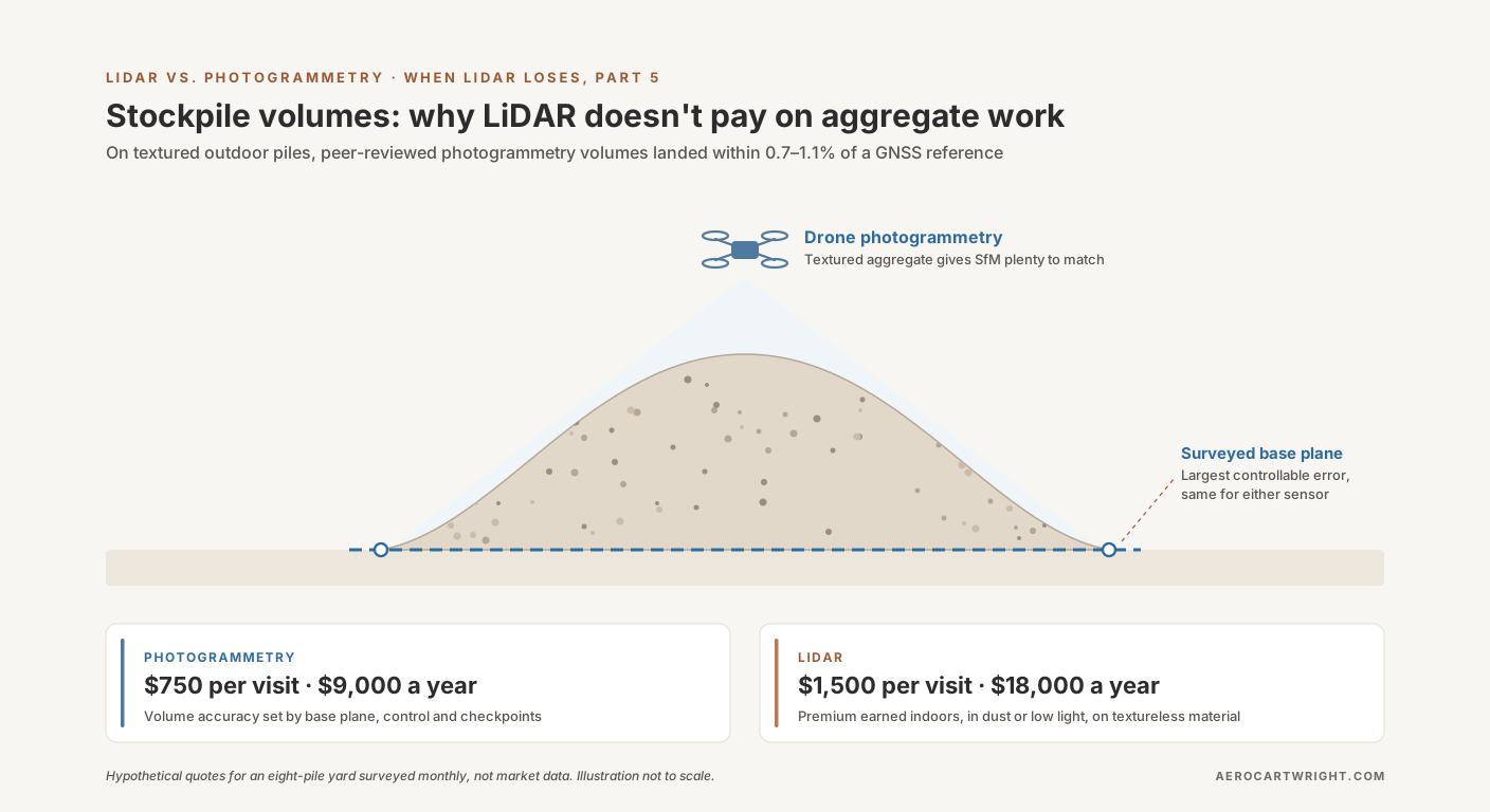
Picture a contractor walking into a sand-and-gravel yard with a quote in hand. Fifteen hundred dollars per visit, monthly, for stockpile volumetrics on an eight-pile yard. His pitch: he flies a Light Detection and Ranging (LiDAR) payload, a DJI Zenmuse L2 on a Matrice 350, and the photogrammetry-only operator quoting seven-fifty for the same scope is selling a less defensible number.
The producer wants a straight answer to the LiDAR vs photogrammetry stockpile question. Is the LiDAR contractor’s nine-thousand-dollar-a-year premium buying a more accurate volume, a more defensible audit trail, or a heavier sensor that doesn’t change the answer?
Short version: on routine outdoor aggregate work, the published evidence gives no reason to expect drone LiDAR to produce a more accurate pile volume than drone photogrammetry, and in this example LiDAR costs twice as much per visit. The largest error source you control, base-plane definition, is sensor-agnostic. The longer version pulls numbers from two peer-reviewed volume studies and a vendor white paper, a 2025 quarry comparison where a photogrammetry payload’s point cloud beat the newer Zenmuse L2 LiDAR’s, and an honest list of the stockpile sub-cases where LiDAR genuinely earns its premium. That list exists. It’s narrow.
This article is the comparative-economic argument: which sensor, for which job, at what cost. The capture protocol, Ground Control Point (GCP) placement and base-plane definition that make a stockpile number audit-defensible get a summary here, not the full treatment. The broader sensor comparison lives in the LiDAR vs Photogrammetry pillar.
What “Routine Aggregate Work” Means
Scope matters. Not every stockpile job has the same shape, and the argument here only applies to the routine case. Routine aggregate work means:
Site: an outdoor producer’s yard, quarry, or distribution lot. Open to the sky. Hard surface or compacted soil. Lit by daylight for the flight window.
Material: crushed stone, sand and gravel, recycled aggregate, road base, processed rock. Textured, with mineral-color variation across the pile surface. Not powdered cement, not fresh white gypsum, not monochrome industrial product.
Yard size and count: sizes vary widely, and there are a lot of them. The US Geological Survey’s Mineral Commodity Summaries 2025 puts construction sand and gravel at 890 million tons produced in 2024 by an estimated 3,400 companies operating 6,500 pits and more than 200 sales and distribution yards. The crushed stone chapter puts crushed stone at 1.5 billion tons from an estimated 1,400 companies operating 3,500 quarries and more than 180 sales and distribution yards. That is about 10,000 pits and quarries (6,500 + 3,500) plus more than 380 yards (200 + 180), most holding several stockpiles.
Pile count: several active piles per site. The worked example below uses eight.
Cadence: monthly for active inventory yards where material moves daily; quarterly for stable strategic reserves; before-and-after for large deliveries and draw-downs; annually for end-of-year financial reporting.
Accuracy spec: Raeva and colleagues (cited below) note that in some countries mine-engineering legislation requires stockpile volumes within plus or minus 3%, and they worked to that target. Your contract or auditor sets your tolerance. Ask what it is before paying to beat it.
Inside that scope sits the routine case: the same yard, the same piles, every month. That repetition is why a per-visit cost difference matters. It recurs twelve times a year.
Sites outside that scope — indoor salt domes, cement clinker barns, fugitive-dust active blast areas, statewide Department of Transportation (DOT) inventory programs — get covered in the LiDAR-wins section below. The next several sections are only about the routine case.
Photogrammetry’s Stockpile Numbers — What the Studies Measured
The accuracy case for photogrammetry on textured outdoor stockpiles rests on one vendor white paper and two peer-reviewed studies.
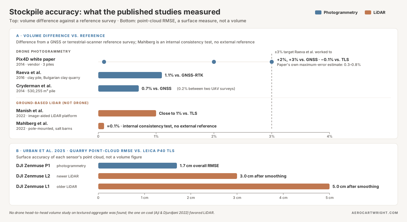
Pix4D white paper (vendor, 2014). Pix4D’s white paper by Bernhard Draeyer and Christoph Strecha compared Pix4D volumes for three piles against GNSS or terrestrial-laser-scanner surfaces and measured differences of +2%, +3% and −0.1%. From a mean surface deviation of −2 to +4 cm, the authors then estimated a maximal volume error of 0.3–0.8% of the total volume, and call that estimate “very simplistic” and specific to their test. Vendor source. Treat it with appropriate skepticism and lean on the independent work below.
Raeva, Filipova & Filipov 2016. In ISPRS Archives XLI-B1, the team flew an eBee Unmanned Aerial Vehicle (UAV) over a Bulgarian open-pit clay quarry and compared the volume of one stockpile of the excavated clay against a Global Navigation Satellite System Real-Time Kinematic (GNSS-RTK) survey. The UAV volume came out 143.99 m³ higher, a 1.1% difference. The UAV flight covering the whole quarry took under 28 minutes; the GNSS survey took about an hour and a half for the stockpile alone and more than five hours for the quarry berms. The authors note that some countries’ mine-engineering legislation requires plus or minus 3%. UAV photogrammetry sat well inside that.
Cryderman, Mah & Shufletoski 2014. In Geomatica 68(4):309–317, UAV photogrammetry volumes on a 530,255 m³ pile agreed with a conventional GNSS survey within 3,755 m³ (0.7%). Two UAV surface models of the same pile, flown with different ground control at different times, agreed within 877 m³ (0.2%). The authors found UAV positional accuracies very similar to GNSS RTK at the scale of photography flown.
The two peer-reviewed studies landed within 0.7% and 1.1% of a GNSS reference. The vendor paper’s three piles ranged from 0.1% to 3%. All of it sits inside the plus-or-minus-3% target Raeva and colleagues worked to, on outdoor stockpiles with ground control. Raeva’s pile was clay, not crushed aggregate, so it supports the outdoor-stockpile case in general rather than aggregate specifically.
The quotable line:
Cryderman 2014 got 0.7% against GNSS on a 530,000 m³ pile. Raeva 2016 got 1.1% on a clay stockpile. Pix4D’s own white paper measured 0.1% to 3% on three piles. That is the band LiDAR would have to beat, and we found no published study showing it does on textured aggregate.
Honest summary on stockpile drone accuracy: on a textured outdoor pile, with a sound methodology (high overlap, grid plus oblique capture, surveyed GCPs around the pile perimeter, a surveyed or perimeter-defined base plane, and independent checkpoints), the published photogrammetry results sit between 0.1% and 3%, with both peer-reviewed studies at about 1% or better. The constraint isn’t the sensor. It’s the protocol.
Does LiDAR Actually Move the Number?
Intuition says more points, active illumination, and direct range measurement should produce a more accurate volume. The published data doesn’t show that on textured outdoor aggregate.
What the outdoor LiDAR volume evidence looks like. Drone-LiDAR service providers and resellers advertise percent-level volume accuracy on outdoor stockpiles, but those are marketing claims. We found no peer-reviewed study that flies drone LiDAR and drone photogrammetry over the same textured aggregate piles and compares both volumes against an independent reference. The one drone head-to-head volume study we found was on coal: Aji & Djurdjani 2022 (JGISE 5(2):132–138) measured a coal stockpile in East Kalimantan, Indonesia, and the LiDAR volume came within 1.426% of a GPS survey against 2.338% for photogrammetry, with 2% (ASTM D6172-98) as their tolerance. Their photogrammetry used direct georeferencing (camera positions from the drone’s GPS/INS, no ground control points), so it is not a like-for-like test of the GCP-controlled photogrammetry in the studies above. The authors recommend LiDAR for coal and blame photogrammetry’s miss on under- and over-exposed images of a homogeneous surface. That is the coal exception covered below, not textured aggregate. Without an aggregate study, there is no evidence of a clean “1% LiDAR versus 3% photogrammetry” gap on textured piles.
Urban et al. 2025 — the quarry test that inverts the assumption. Urban, Štroner and colleagues (European Journal of Remote Sensing 58) compared point clouds from three DJI sensors over the same quarry against a Leica P40 terrestrial laser scanner reference. These are point-cloud accuracy figures, not volume errors. From the paper’s abstract:
| Sensor | Type | Point-cloud RMSE vs TLS reference |
|---|---|---|
| DJI Zenmuse P1 | Photogrammetry | 0.017 m (1.7 cm), overall |
| DJI Zenmuse L2 | LiDAR (newer generation) | 0.03 m (3.0 cm), after smoothing |
| DJI Zenmuse L1 | LiDAR (older generation) | 0.05 m (5.0 cm), after smoothing |
The quotable line for the next sales conversation:
In the Urban et al. 2025 quarry comparison, the DJI Zenmuse P1 photogrammetric point cloud was more accurate than the newer Zenmuse L2 LiDAR cloud: 1.7 cm overall RMSE vs 3.0 cm after smoothing, against a terrestrial-scanner reference.
Read it carefully. The authors call the photogrammetric cloud “still somewhat better”, conclude that the L2’s accuracy “is sufficient for a vast majority of applications,” and add that “the new generation scanning technology has the potential to replace photogrammetry” for UAV point clouds. The study compared the L2 with the older L1; DJI’s newer Zenmuse L3 was not tested. This is not a verdict that LiDAR is bad. It is evidence that on exposed quarry rock, the L2 does not buy a more accurate surface than photogrammetry, and a more accurate surface is the only route by which a sensor could buy a more accurate volume.
The base-plane problem is the one neither sensor solves. Stockpile volume is the integral of pile-surface elevation minus base-plane elevation over the pile footprint, so a base-plane offset multiplies straight across the footprint. Get the base plane wrong by 2 cm on a 5,000 m² pile and the volume is wrong by 100 m³ (0.02 m × 5,000 m²), about 131 yd³. At an assumed $30/yd³ for aggregate, that’s about $3,900 of disputed material per pile, scaling linearly with footprint. An automatically detected base plane is the part of the workflow to distrust. The audit-defensible approach is a surveyed pad or a perimeter-elevation polygon.
LiDAR’s headline spec is point rate. DJI lists the Zenmuse L2 at a 240 kHz pulse rate, with up to 240,000 points per second single-return and 1.2 million points per second multi-return. Density and base-plane definition are different problems. A wrong base plane stays wrong at any density. A denser cloud produces a sharper-looking edge on the same wrong volume.
The base-plane error doesn’t change when you switch sensors. Full stop.
The Anchor Accuracy Table
| Source | Year | Setting | Reference | Sensor | Result |
|---|---|---|---|---|---|
| Pix4D white paper (vendor) | 2014 | Three outdoor piles | GNSS / TLS | Photogrammetry | 0.1%, 2%, 3% volume difference (paper’s estimated maximum error 0.3–0.8%) |
| Raeva et al. (ISPRS Archives) | 2016 | Clay stockpile, open-pit clay quarry, Bulgaria | GNSS-RTK | Photogrammetry | 1.1% volume difference |
| Cryderman et al. (Geomatica) | 2014 | 530,255 m³ pile | Conventional GNSS survey | Photogrammetry | 0.7% volume difference; 0.2% UAV-to-UAV |
| Urban et al. (EJRS 58) | 2025 | Quarry | Leica P40 TLS | P1 / L2 / L1 | Point-cloud RMSE: P1 1.7 cm overall; L2 3.0 cm and L1 5.0 cm after smoothing (not a volume figure) |
| Aji & Djurdjani (JGISE 5) | 2022 | Coal stockpile, Indonesia | GPS survey | Drone LiDAR vs photogrammetry (directly georeferenced, no GCPs) | LiDAR 1.426%, photogrammetry 2.338% volume difference |
| Manish et al. (Rem. Sens. 14:231) | 2022 | Stockpiles, image-aided LiDAR platform | TLS | Ground-based LiDAR | Close to 1% relative volume error |
| Mahlberg et al. (Rem. Sens. 14:4802) | 2022 | Salt storage barns | Conservation-of-volume test | Pole-mounted LiDAR | About 0.1% |
The Pix4D entry is a vendor source. The two LiDAR volume rows are ground-based systems, not drone LiDAR outdoors; they are the evidence for the LiDAR-wins cases later in the article. Urban 2025 compares point-cloud accuracy, not volumes. Aji & Djurdjani is the only drone head-to-head volume study we found; it is on coal, where LiDAR is expected to win, and its photogrammetry used direct georeferencing without GCPs.
Why Aggregate Is Photogrammetry’s Home Court
Crushed aggregate isn’t a neutral test surface. It’s close to an ideal one for SfM. The underlying mechanism explains why the accuracy numbers in the previous section came out the way they did.
Crushed aggregate is rich in texture. Crushed stone, raw aggregate, and sand-and-gravel piles carry micro-texture: corners, edges, mineral color variation, shadow patterns. Structure from Motion (SfM) builds its surface by matching distinctive features between overlapping photos, and a textured pile gives it plenty to match.
LiDAR’s advantages are real. They just show up on different surfaces and in different conditions: through canopy gaps, through dust, in low light, on monochrome material. On open textured aggregate, the surface itself hands photogrammetry what it needs.
Then there’s the orthomosaic. A photogrammetric flight produces an orthomosaic and textured mesh as a structural by-product. A LiDAR return carries no photo texture, so producing either from a LiDAR job means flying a Red-Green-Blue (RGB) camera alongside it and processing that imagery. For stockpile reporting, where the report gets read by a quarry manager, a Chief Financial Officer, or an auditor, visual deliverables matter. A photo-accurate top-down view with pile annotations beats a colored point cloud for the audience that signs off on the number.
The monochrome exception. SfM fails on uniform surfaces. Powdered cement, fresh white gypsum, lime, dry uniform white sand: tie-point matching produces sparse or interpolated point clouds that look like data and aren’t. On a flat surface you can scatter high-contrast markers before flight. On a working cement clinker pile, that’s neither practical nor safe. For monochrome material, LiDAR is the right sensor. That case lives in the LiDAR-wins section below.
For everything else — outdoor textured aggregate, daylight, accessible to a multirotor — the structural argument is photogrammetry’s.
The Per-Visit Cost Math
The accuracy argument narrows the discussion: on routine aggregate work, nothing in the published record shows LiDAR buying a better volume. From there, the question is cost.
Hardware and software, with dated prices. The DJI Mavic 3 Enterprise, the long-time small mapping drone, is discontinued: dealer Global Drone HQ lists it as no longer available (last listed at $4,950) and names the Matrice 4E, at $5,189, as its direct replacement (checked October 2, 2026). Processing software runs from free (WebODM, OpenDroneMap) through Pix4Dmapper at $3,990 a year ($332.50 a month billed yearly) to Agisoft Metashape Professional at $3,499 perpetual (both checked October 1, 2026). DJI does not publish US prices for the Matrice 350 RTK or the Zenmuse L2 payload, so price that stack from dealer quotes.
Since September 3, 2026, most imported drones carry an added Section 232 duty: 25% for aircraft without thermal imaging (which covers the Mavic 3E and Matrice 4E), and up to 100% for thermal-equipped aircraft and some other categories. Lower rates apply to some trading partners, and component duties phase in on February 9, 2027. Confirm whether a dealer’s listed price already includes the duty. For the producer, none of this changes the decision. The producer is buying visits, not hardware.
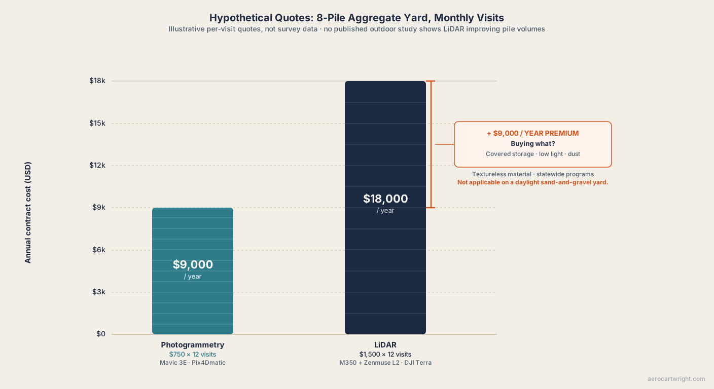
Here is a paired worked example for the contractor at the producer’s door. It is a hypothetical: the quotes match the opening scene, and the field and processing times are illustrative planning assumptions, not measurements.
Example A (hypothetical): 8 piles, monthly captures, photogrammetry.
- Drone: DJI Mavic 3E, or its replacement, the Matrice 4E
- Software: Pix4Dmatic (or Pix4Dmapper subscription)
- Field time: ~45 min flight + 30 min GCP work
- Processing: ~2 hours on a workstation
- Operator pricing: $750 per visit (hypothetical quote)
- Yearly contract: $9,000 ($750 × 12)
- Accuracy: set by the base plane, ground control and checkpoints, as in the studies above
Example B (hypothetical): same site, LiDAR contractor.
- Drone: DJI Matrice 350 RTK + Zenmuse L2
- Software: DJI Terra (boresight, trajectory) plus classification and Digital Terrain Model (DTM) extraction
- Field time: ~30 min flight (single nadir pass, faster) + 30 min GCP work
- Processing: ~3 hours (boresight calibration, Smoothed Best Estimate of Trajectory (SBET) processing, strip alignment, classification, DTM)
- Operator pricing: $1,500 per visit (hypothetical quote, twice Example A)
- Yearly contract: $18,000 ($1,500 × 12)
- Accuracy: set by the same base plane, ground control and checkpoints
The delta. No published evidence shows B producing a more accurate volume than A on this yard. Cost delta: ($1,500 − $750) × 12 = +$9,000 per year for the same audit-defensible number. On the producer’s yard, the LiDAR contractor’s only honest pitch is “I can fly it at dusk and in dust.” True. Rarely the binding constraint on a daylight sand-and-gravel yard.
The quotable line:
The honest LiDAR pitch on aggregate isn’t ‘more accurate volume.’ It’s ‘covered storage, dust, low light, monochrome material, statewide inventory programs.’ For everything else, photogrammetry meets the spec, and in this example at half the per-visit price.
That list of sub-cases is the next section, and it is non-negotiable.
When LiDAR Earns Its Premium on Stockpile Work
The argument above only holds if its boundary is honest. The boundary is real. There are stockpile sub-cases where LiDAR is the right sensor — full stop — and the producer on one of those sites should pay the premium.
Indoor and confined storage. Salt domes, cement clinker barns, gypsum sheds, lime warehouses, covered aggregate barns. Global Positioning System (GPS) denied, often dust-loaded, frequently dark. Photogrammetry needs ambient light and surface texture. LiDAR carries its own light source, so darkness doesn’t stop it, and the cement-silo case below shows it working in dusty storage.
The documented technical evidence. Note that both peer-reviewed studies used ground-based LiDAR, not a drone:
- Mahlberg, Manish, Koshan, Joseph, Liu, Wells, McGuffey, Habib & Bullock 2022 (Remote Sensing 14(19):4802, “Salt Stockpile Inventory Management Using LiDAR Volumetric Measurements”) describe a portable pole-mounted LiDAR that can inventory a large salt barn in under 15 minutes and was deployed over 90 times at 30 facilities. A conservation-of-volume test, repositioning portions of a salt pile, indicated volumes accurate to approximately 0.1%.
- Manish, Hasheminasab, Liu, Koshan, Mahlberg and colleagues 2022 (Remote Sensing 14(1):231, “Image-Aided LiDAR Mapping Platform and Data Processing Strategy for Stockpile Volume Estimation”) built the Stockpile Monitoring and Reporting Technology (SMART) platform, fusing camera and LiDAR data for conditions with no GNSS signal, poor lighting or featureless surfaces. Against terrestrial laser scanner reference volumes, it came in close to 1% relative error.
- Flyability Elios 3 at a French cement plant (vendor case, reported by Geo Week News): a LiDAR-equipped indoor drone measured clinker stored in silos, replacing a worker probing the pile with a pole. No accuracy figure is published there. It shows the use case, not the error bar.
Low-light and dusty operations. Active quarry blast areas, plants running 24/7, fugitive-dust environments, dawn or dusk loading operations. Photogrammetry needs light: as it fades, exposure times lengthen and image quality and tie-point matching suffer. LiDAR doesn’t depend on ambient light. If the operational window is “we run regardless of daylight,” LiDAR holds spec.
Monochrome and textureless material. Powdered cement, fresh white gypsum, lime, fresh white sand, dry uniform fly ash. Feature matching has little to grab on uniform surfaces. The resulting SfM cloud is sparse and interpolated, and not measurable to engineering tolerance. LiDAR measures range directly instead of matching texture.
Coal and dark, uniform surfaces. Dark, homogeneous surfaces give SfM little contrast to match, so the same mechanism applies by reasoning. Here there is a direct test: Aji & Djurdjani 2022 flew drone LiDAR and drone photogrammetry over a coal stockpile and compared both with a GPS survey. LiDAR came within 1.426%, photogrammetry 2.338%, against the 2% tolerance they took from ASTM D6172-98. Their photogrammetry was directly georeferenced, with no ground control points. The authors put photogrammetry’s miss down to under- and over-exposed photos of a homogeneous surface and recommend LiDAR for coal.
Statewide recurring inventory programs. Mahlberg, Malackowski, Joseph, Koshan, Manish, DeLoach, Habib & Bullock 2024 (Remote Sensing 16(2):410, “Statewide Implementation of Salt Stockpile Inventory Using LiDAR Measurements: Case Study”) documented the Indiana DOT rollout: a portable pole-mounted LiDAR at about 120 salt storage facilities, an end-of-season inventory in 9 working days with two INDOT staff members, and volumes delivered within 24 hours of data collection. The scanner amortizes against a recurring institutional program where photogrammetry’s lighting and access dependencies become operational liabilities. A DOT that needs guaranteed delivery inside covered storage pays the LiDAR premium and gets it back in schedule reliability.
We found no published count of how many stockpile jobs fall into these five sub-cases. On a plain reading of the scope above, they are the minority. The rest (outdoor textured aggregate, lit reasonably, accessible to a multirotor) is photogrammetry’s territory, and the LiDAR premium isn’t earned there. The minority is real, though. A producer with a clinker silo or a DOT salt-barn contract should buy the LiDAR pitch, not the photogrammetry pitch. Honesty about scope is what makes the photogrammetry argument credible everywhere else.
Audit Defensibility — Same With or Without LiDAR
When accuracy and cost don’t land, the fallback pitch is audit defensibility. The argument: when this number gets challenged, the operator who flew LiDAR has a more defensible deliverable. That argument is wrong, and it matters. Audit defensibility is the most commercially valuable framing in stockpile work.
A defensible stockpile deliverable requires:
- Documented capture protocol — altitude, overlap, pattern (grid plus oblique), weather
- Surveyed GCPs with audit-traceable coordinates, survey method, and occupation time
- Defined base plane with documented source (surveyed pad, custom perimeter polygon with elevations, or best-fit with rationale)
- Checkpoint validation with measured horizontal RMSE (RMSEH) and vertical RMSE (RMSEV) residuals, with the checkpoint count stated in the report
- A conservative accuracy claim matching the measured residuals
- Period-over-period methodology locked from capture one
- Raw data preservation for the audit period
None of those items is sensor-specific. Every line on that list applies to a photogrammetry deliverable and a LiDAR deliverable equally. The methodology gets defended in deposition, not the point cloud.
The LiDAR deliverable actually carries more audit overhead, not less. A defensible LiDAR report includes everything above plus:
- Boresight calibration logs (sensor-to-Inertial Measurement Unit (IMU) alignment)
- SBET smoothing parameters and quality metrics
- Strip alignment results across flight lines
- Ground point classification methodology and quality control
- DTM extraction parameters and ground-class verification
Each is a step the operator has to be prepared to defend under cross-examination. None of them reduces the number of methodology questions the deposition will ask. All of them add to it.
The quotable line:
Switching sensors doesn’t reduce litigation risk. The audit defends the methodology, not the point cloud.
The deposition question is “describe your methodology for determining the base plane on this pile.” The answer is either “we surveyed the pad before the pile was placed and reused the surveyed base plane across all twelve captures” or it isn’t. The drone in the air doesn’t change the answer. The Ground Control Points for Drone Surveys and RTK vs PPK for Drone Mapping articles cover the upstream control work that makes the answer defensible regardless of sensor.
The methodology is portable across sensors. The sensor isn’t what gets defended.
Closing — What the Producer Should Ask the Contractor
Back to the producer at the door. A LiDAR contractor with a $1,500-per-visit quote, a photogrammetry operator with a $750-per-visit quote, both proposing to measure the same eight piles on the same yard, monthly.
Ask five questions.
“What is your base-plane methodology?” If the answer is “surveyed pad” or “perimeter polygon with surveyed elevations,” the operator is competent regardless of sensor. If the answer is “whatever the software detects automatically,” walk away regardless of sensor. The largest controllable error source isn’t the drone in the air.
“What is your checkpoint RMSE expectation, and how is it measured?” If the answer references surveyed checkpoints not used in the bundle adjustment, with reported RMSEH and RMSEV, the deliverable is defensible. If the answer is “the software said it was accurate,” it isn’t.
“What is your accuracy claim, and what is it conditional on?” A claim near 1% is consistent with the peer-reviewed results above, but only with a surveyed base plane, surveyed control and checkpoint residuals to back it. A blanket 1% claim with no conditions is marketing copy.
“What is your period-over-period methodology lock?” Same flight altitude, same overlap, same GCP locations, same base plane, same software. An operator who can’t answer this won’t compare apples-to-apples between the first capture and the second.
“What does my deliverable include — orthomosaic, DSM, point cloud, audit report?” The photogrammetry deliverable includes an orthomosaic and textured mesh as structural by-products. The LiDAR-only deliverable doesn’t, unless the operator paired the LiDAR with a synchronized RGB camera and ran a parallel photogrammetric pipeline. That adds cost.
The sensor isn’t on the list. None of those questions are answered better by LiDAR on a routine textured outdoor aggregate yard. The answers are about the operator’s methodology, which is sensor-portable, and the deliverable structure, which favors photogrammetry on outdoor work.
The quotable closing line:
For routine outdoor aggregate work, the drone in the air matters less than the GCPs on the ground and the base plane in the software. Photogrammetry handles the air; the methodology handles the rest. LiDAR doesn’t change that calculus.
That’s the producer’s answer. The $9,000-per-year premium for LiDAR on a textured outdoor yard isn’t buying a more accurate number, isn’t buying a more defensible audit trail, and isn’t buying a deliverable the auditor reads differently. It’s buying low-light capability the daylight yard doesn’t need, monochrome-material capability the yard doesn’t have, and indoor coverage the yard doesn’t need. In a clinker silo, a salt barn, or a statewide DOT program, the premium is earned. On a sand-and-gravel yard in daylight, it isn’t.
The broader sensor comparison lives in the LiDAR vs Photogrammetry pillar.
The drone in the air matters less than the methodology on the ground. That’s the entire argument.
References
Research and standards cited in this article.
- Aji, A. R. S., & Djurdjani, D. (2022). Perbandingan volume stockpile batu bara hasil UAV fotogrametri dan UAV lidar [Comparison of coal stockpile volumes from UAV photogrammetry and UAV lidar]. JGISE: Journal of Geospatial Information Science and Engineering, 5(2), 132–138. doi:10.22146/jgise.78295
- Cryderman, C., Mah, S. B., & Shufletoski, A. (2014). Evaluation of UAV photogrammetric accuracy for mapping and earthworks computations. Geomatica, 68(4), 309–317. doi:10.5623/cig2014-405
- Mahlberg, J., et al. (2022). Salt stockpile inventory management using LiDAR volumetric measurements. Remote Sensing, 14(19), 4802. doi:10.3390/rs14194802
- Mahlberg, J., et al. (2024). Statewide implementation of salt stockpile inventory using LiDAR measurements: Case study. Remote Sensing, 16(2), 410. doi:10.3390/rs16020410
- Manish, R., et al. (2022). Image-aided LiDAR mapping platform and data processing strategy for stockpile volume estimation. Remote Sensing, 14(1), 231. doi:10.3390/rs14010231
- Raeva, P. L., Filipova, S. L., & Filipov, D. G. (2016). Volume computation of a stockpile – a study case comparing GPS and UAV measurements in an open pit quarry. International Archives of the Photogrammetry, Remote Sensing and Spatial Information Sciences, XLI-B1, 999–1004. doi:10.5194/isprs-archives-XLI-B1-999-2016
- U.S. Geological Survey. (2025). Mineral commodity summaries 2025. U.S. Geological Survey. doi:10.3133/mcs2025
- Urban, R., et al. (2025). Testing the accuracy and characteristics of data acquired using DJI Zenmuse L1 and L2 lidar systems and photogrammetric data acquired using DJI Zenmuse P1 in a quarry environment. European Journal of Remote Sensing, 58(1), 2595361. doi:10.1080/22797254.2025.2595361