You’re reviewing a construction site survey. The client sent over a single aerial photo — looks great, high resolution, you can see individual rebar on the slab. Then you try to measure the distance between two column footings. The scale changes across the frame. The building leans to the left. The measurement is off by two meters.
That’s the problem an orthomosaic solves. And if you’ve been handing clients individual drone photos instead of orthorectified mosaics, you’ve been handing them pictures — not maps.

What an Orthomosaic Actually Is
An orthomosaic is a georeferenced, orthorectified image mosaic assembled from overlapping aerial photographs. Three words matter in that definition.
Georeferenced means every pixel is tied to a real-world coordinate — latitude, longitude, and usually elevation. You can drop the file into ArcGIS Pro or QGIS and it lands exactly where it belongs on the Earth’s surface, aligned with your other spatial data.
Orthorectified means the geometric distortions in each source image — camera tilt, lens distortion, and terrain relief displacement — have been mathematically removed. The result is a true orthographic projection: a perfectly top-down view where scale is uniform across the entire image.
Mosaic means the individual corrected images have been seamlessly stitched, color-balanced, and blended into a single continuous image covering the full project area.
The result is a map-quality image product where you can measure distances, calculate areas, and extract coordinates directly. A regular aerial photo lets you see what’s on the ground. An orthomosaic lets you measure it.
How Photogrammetry Builds an Orthomosaic
You don’t press a button and get an orthomosaic. The process has distinct computational stages, and understanding them explains why flight parameters matter so much.
Image Capture and Overlap
The drone flies a grid pattern, capturing images with 75 to 85 percent frontal overlap and 65 to 75 percent side overlap. Every point on the ground appears in multiple images from different angles. That redundancy is the raw material photogrammetry needs — without it, the math doesn’t converge.
Tie Point Matching and Bundle Adjustment
Photogrammetry software — Pix4D, Metashape, WebODM, ArcGIS Reality — identifies matching features across overlapping images. These tie points establish geometric relationships between every image pair. Bundle adjustment then solves simultaneously for the precise position and orientation of every camera at the moment each image was captured, plus the 3D location of every tie point. This is a large least-squares optimization, and it’s where your ground control points (GCPs) constrain absolute accuracy.
Dense Point Cloud and Digital Surface Model
With camera positions locked, the software generates a dense 3D point cloud by matching pixels across image pairs at much higher density than the initial tie points. This point cloud gets interpolated into a digital surface model (DSM) — a continuous elevation grid representing the terrain and everything on it.
Orthorectification
Here’s where the correction happens. Each source image is reprojected onto the DSM, removing the perspective distortion caused by camera tilt and terrain relief. Imagine draping each photograph over the 3D surface model and viewing it from directly above. Objects that appeared to lean in the original photos are corrected to their true planimetric positions. The math accounts for every meter of elevation change across the site.
Mosaicking and Color Balancing
The individual orthorectified images — now called orthophotos — get stitched along computed seam lines that avoid cutting through objects. Color balancing normalizes brightness and contrast across images captured at slightly different sun angles or exposures. The output is one seamless, georeferenced image.

Ground Sample Distance: What Resolution Actually Means
Ground sample distance (GSD) is the real-world size of one pixel in your orthomosaic. A 2 cm/pixel GSD means each pixel covers a 2 cm by 2 cm area on the ground. That’s your resolution floor — you cannot reliably identify features smaller than roughly 2 to 3 times your GSD.
The formula is straightforward:
GSD = (Sensor Width x Flight Height) / (Focal Length x Image Width in Pixels)
In practice, GSD is controlled by flight altitude. Fly lower, get finer resolution. Fly higher, cover more area per flight line but lose detail. Most professional drone mapping projects target 1 to 3 cm/pixel.
| Flight Altitude | Typical GSD (20mm lens, full-frame) | Use Case |
|---|---|---|
| 30 m (100 ft) | ~0.8 cm/px | Structural inspection, crack detection |
| 60 m (200 ft) | ~1.5 cm/px | Construction monitoring, stockpile volumes |
| 80 m (260 ft) | ~2.0 cm/px | General site survey, boundary mapping |
| 120 m (400 ft) | ~3.0 cm/px | Large-area agriculture, environmental |
GSD matters because it sets the measurement precision ceiling. A 3 cm/pixel orthomosaic cannot reliably resolve a 5 cm crack — the feature is barely larger than a pixel. Match your GSD to the smallest feature you need to detect.
File Formats: GeoTIFF, COG, and ECW
An orthomosaic is a raster file — a grid of pixels with embedded spatial reference information. The format you export determines file size, compatibility, and how efficiently it can be served.
GeoTIFF is the universal standard. Every GIS platform, CAD tool, and web mapping service reads GeoTIFF. The file embeds coordinate reference system metadata, so the software knows exactly where to place it. Uncompressed GeoTIFFs for large sites routinely hit 5 to 20 GB. LZW or DEFLATE compression cuts that significantly without quality loss.
Cloud Optimized GeoTIFF (COG) is a GeoTIFF with internal tiling and overviews arranged so that a client application can request just the tiles and zoom levels it needs via HTTP range requests — without downloading the entire file. COG is now an official OGC standard. If you’re serving orthomosaics through a web portal, cloud storage, or STAC catalog, COG is the format. Every COG is a valid GeoTIFF, so backward compatibility is built in.
ECW (Enhanced Compression Wavelet) achieves roughly 15:1 compression versus GeoTIFF’s typical 8:1, producing significantly smaller files with minimal visible quality loss. The tradeoff: ECW is a proprietary format owned by Hexagon. Reading ECW is free in most software, but writing requires a license. Government agencies and large engineering firms still use ECW heavily for distribution.
The practical decision: Export your master archive as uncompressed or lossless GeoTIFF. Distribute to GIS users as COG. If your client’s CAD team demands small files and uses Hexagon software, ECW. For web maps and dashboards, COG served through a tile server or cloud storage.
Coordinate Systems and Accuracy
Every orthomosaic carries a coordinate reference system (CRS) — the mathematical model that maps pixel locations to positions on the Earth. Most photogrammetry software exports in WGS 84 / UTM by default, identified by an EPSG code (for example, EPSG:32617 for UTM Zone 17N).
If your client needs the deliverable in a state plane coordinate system — say NAD83 / Florida East (EPSG:2236) — you reproject the raster in your GIS software using the appropriate datum transformation. Do not manually edit the CRS metadata. Use the Project Raster tool in ArcGIS Pro or gdalwarp from the command line. Changing metadata without reprojecting shifts every coordinate.
Positional Accuracy
The ASPRS Positional Accuracy Standards for Digital Geospatial Data define accuracy using root mean square error (RMSE) measured against independent checkpoints. A project that achieves 5 cm horizontal RMSE belongs to the ASPRS 5 cm accuracy class. The current edition requires a minimum of 30 independent checkpoints for formal accuracy assessment.
For typical drone orthomosaics:
| Positioning Method | GCPs Used | Expected Horizontal RMSE |
|---|---|---|
| RTK/PPK + GCPs | Yes (5+) | 1–3 cm |
| RTK/PPK only | No | 3–8 cm |
| Standard GNSS (no corrections) | No | 1–5 m |
| Standard GNSS + GCPs | Yes (5+) | 3–5 cm |
Accuracy is not resolution. A 1 cm/pixel orthomosaic with no ground control is high-resolution but low-accuracy — the pixels are sharp, but they might be in the wrong place by several meters. GSD tells you what you can see. Accuracy tells you where it actually is. Conflating the two is one of the most common mistakes in drone deliverables.
How to Use an Orthomosaic in GIS
Loading an orthomosaic into ArcGIS Pro or QGIS is straightforward — drag the GeoTIFF into the map canvas and it reprojects on the fly to match your project CRS. But using it effectively takes more than just looking at pretty pixels.
Measurement and Digitization. With the orthomosaic as your basemap, you can digitize features directly — building footprints, road centerlines, stockpile boundaries, vegetation zones. The measurements are spatially accurate to the precision of the orthomosaic’s positional accuracy and GSD.
Change Detection. Fly the same site on a regular schedule and stack the orthomosaics temporally. Pixel-by-pixel comparison reveals earthwork progress, vegetation encroachment, erosion, or structural changes. This is standard practice on construction sites — weekly flights compared against design surfaces.
Integration with Other Layers. Orthomosaics sit in the same coordinate space as your parcels, utilities, contours, and design files. Overlay a CAD site plan on the orthomosaic and you see immediately whether the as-built matches the design. That visual check catches errors that coordinate-only comparisons miss.
Classification and Analysis. Multispectral orthomosaics support vegetation index calculations — NDVI, NDRE, SAVI — directly in the raster. RGB orthomosaics can be classified using supervised or unsupervised methods to delineate land cover types, impervious surfaces, or crop species.
Real-World Applications by Industry
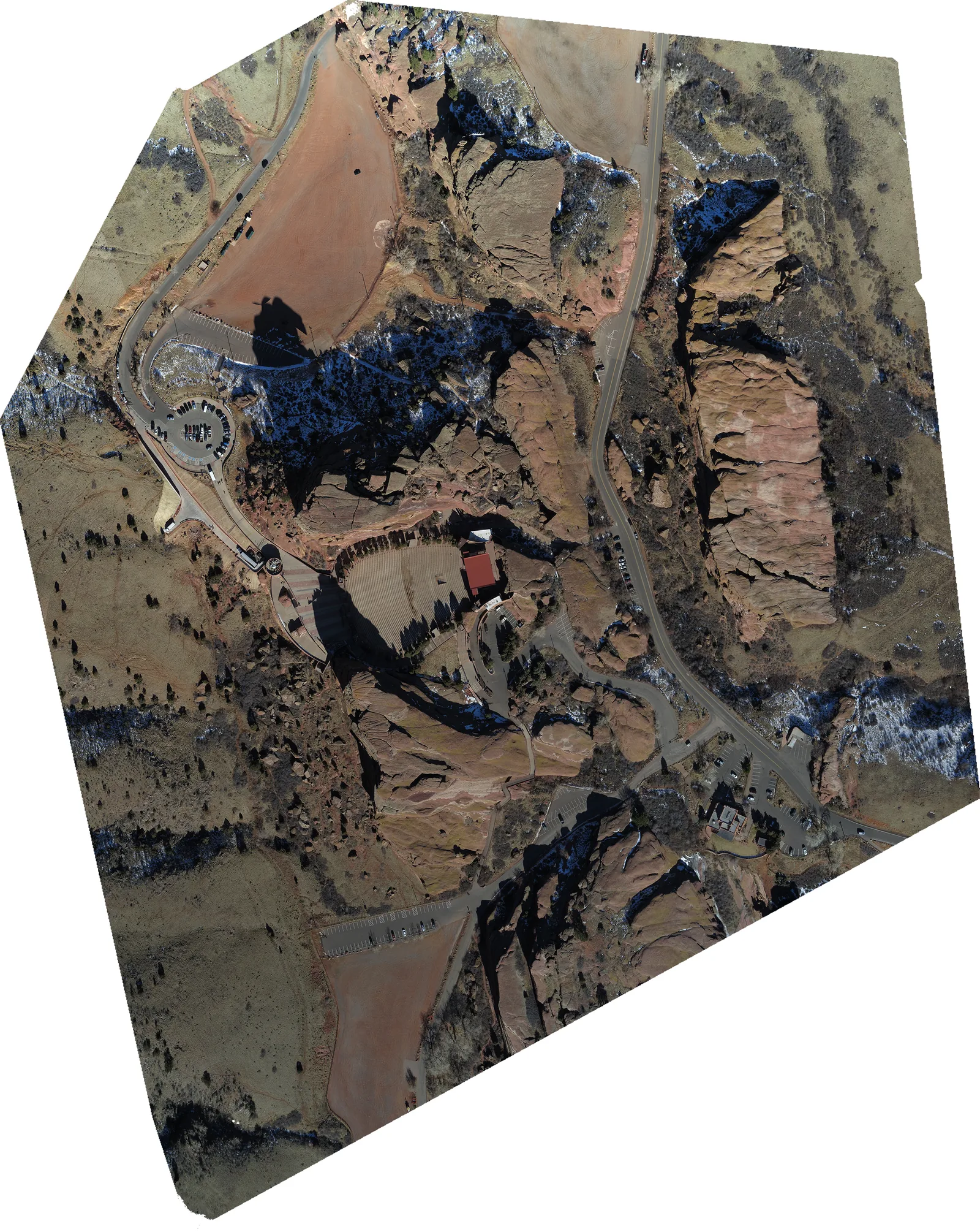 “Geo-referenced Orthomosaic of Red Rocks” by Stoermerjp (DroneMapper.com / Falcon UAV), via Wikimedia Commons, CC BY-SA 3.0
Construction. Weekly orthomosaics track earthwork progress, verify as-built conditions against design surfaces, and calculate cut/fill volumes when combined with DSMs. Project managers overlay orthomosaics on BIM models to identify deviations before they become expensive rework. One orthomosaic replaces dozens of ground-level progress photos and gives the entire team a common spatial reference.
Land Surveying. Orthomosaics serve as the visual layer beneath survey-grade point data. Boundary surveys use them to identify physical occupation — fences, driveways, structures — relative to legal boundaries. Topographic surveys combine orthomosaics with contour data for complete site documentation. The deliverable is more intuitive to clients who don’t read contour maps.
Agriculture. Multispectral orthomosaics reveal crop stress invisible to the naked eye. A farmer comparing NDVI values across a 500-acre field identifies irrigation failures, nutrient deficiencies, and pest damage at the individual-row level. Temporal stacking across the growing season quantifies yield variability and informs variable-rate application maps.
Environmental and Natural Resources. Wetland delineation, shoreline erosion monitoring, wildfire damage assessment, habitat mapping — all rely on high-resolution, georeferenced imagery as the spatial backbone. Regulatory agencies accept drone orthomosaics for permit documentation when accuracy meets ASPRS standards and the coordinate system matches the project datum.

What an Orthomosaic Cannot Do
Orthomosaics are powerful, but they have real limitations worth understanding.
Vertical features distort. Orthorectification corrects ground-level features accurately but above-ground objects — buildings, trees, utility poles — lean away from the camera positions. A true orthomosaic (sometimes called a “true ortho”) corrects for this using a full 3D mesh, but standard DSM-based orthorectification leaves building facades smeared or duplicated along seam lines.
Moving objects ghost. Cars, people, and machinery that change position between overlapping image captures appear as transparent smears — the blending algorithm averages pixels from images where the object was and wasn’t. This is inherent to the mosaicking process.
Shadow and occlusion zones. Tall structures cast shadows that vary between images. The mosaic blends these inconsistently, creating visual artifacts. Areas occluded behind buildings in every image angle produce blank spots or warped fills.
Accuracy depends on the weakest link. A beautiful 1 cm/pixel orthomosaic processed without GCPs and flown on consumer-grade GPS is a high-resolution picture, not a survey-grade map. The processing pipeline cannot manufacture accuracy that the input data doesn’t contain.
Bottom Line
An orthomosaic transforms raw drone photographs into a spatially accurate, measurable map product. The orthorectification process removes the geometric distortions that make individual aerial photos unsuitable for measurement. The georeferencing pins every pixel to real-world coordinates. The result is a deliverable that works as a GIS layer, a measurement surface, and a visual record — all in one file.
The quality of that deliverable depends on flight planning (overlap and GSD), ground control (GCPs and positioning method), and processing parameters. Get those right and the orthomosaic becomes your most versatile drone mapping product. Get them wrong and you have a pretty picture that lies about where things are.
For the positioning methods that control orthomosaic accuracy, see RTK vs PPK Drone Mapping. For ground control strategy, see Ground Control Points for Drone Surveys. For the full flight-to-delivery workflow, see the Complete Drone Mapping Workflow Guide.